Tuesday, July 17, 2018

Open science, Early career researchers and Gender equality!


Recently, there has been an increasing number of protests against the publication science models adopted and ran in North America and Europe. These critics are fundamental to a shift of the paywall systems to a more collaborative and open framework, which will eventually take into account the reassessment and improvement of outdated publication methods, i.e., the peer-review. In this context, it is quite mandatory and useful to read two articles: this one and this other one

In my opinion, Early Career Scientists (ECRs) have a fundamental role in this game-change process. Most mid and late career scientists suffer from a strong inertia that, in turn, will demand too much energy to change their publishing habits (e.g. https://www.theatlantic.com/science/archive/2018/04/the-scientific-paper-is-obsolete/556676/) and will cause no significant selfish individual career improvements. ERCs are usually trapped in many system loopholes, but they often have the choice of targeting the journals to where they want to submit their research, and this makes lots of difference. Thinking out of the box by sharing your data and code is already a game changer, for better. Making use of journals that allow you to share your research in an open and transparent way is undoubtedly the right path to follow. My own experience has shown very positive results. I have been a user of the Open Science Framework (http://osf.io) to share my data and the EarthArXiv (https://eartharxiv.org/) to store my pre and postprints.

All this discussion on open science is especially interesting to me because back in 2009 (when I was doing my masters) I was still living in the “Brazilian scientific way of thinking” bubble. Let me be clearer, in Brazil the vast majority of publications are published in open (and free) access journals. In a nutshell, the Brazilian Government coordinates its own evaluation of scientific journals by attributing a higher impact to national-based journals than they have at an international scale. Although this system is not perfect, it makes a lot of sense since many scientific problems are dealt on a national level (sometimes only local significance) and not in English. Most of these journals are maintained by Universities, societies, and direct government-based funding initiatives. The most renowned example is the Scientific Electronic Library Online (SciELO, www.scielo.org). SciELO indexes, store and offer scientific manuscripts for over 20 years. This platform offers over 700 thousand peer-reviewed manuscripts for free, which have been cited over 15 million times. Given that is not a surprise that Brazil is considered a leader in open science (https://orcid.org/blog/2018/06/18/brazilian-leadership-open-research) and that it has help pushing Latin America in this practice (https://www.timeshighereducation.com/blog/why-open-access-publishing-growing-latin-america).


And it is not only in open access research that Brazil is considered a leader. Not long ago, there was Brazil was also a global leader in gender equality in science (https://www.forbes.com/sites/shannonsims/2017/03/08/surprising-new-study-brazil-now-a-global-leader-in-gender-equality-in-science/#56fc2216f448). These are great news, indeed. As a Brazilian national, I wonder what is the setup/decision tree that provided this outcome. Probably this is the only high profile permanent job (in terms of salary) in Brazil that is considered relatively gender balanced. Is anyone taking notes of these good examples and trying to replicating them in other countries? I’m not aware of it, but it would be good know that good practices are being followed or further improved.

Monday, January 2, 2017

Hydrographs in R

Long time no see.

Well, to feed this blog more often I decided to document some unpublished work I did in the past and also tiny things what could make others' life easier.

Around 3 years ago I wanted to plot hydrographs in R. In my case, I wanted a way that I could automatically generate a sub-hourly hydrograph to show in a very small time scale the rainfall, Q and Qbase.

I was inspired by the graphs in this very interesting paper: Aich, V., Zimmermann, A., Elsenbeer, H., 2014. Quantification and interpretation of suspended-sediment discharge hysteresis patterns: How much data do we need? Catena 122, 120–129. doi:10.1016/j.catena.2014.06.020

I found a package in R what did exactly what I wanted. The name of the package is EcoHydRology. This package is very nice, but the hydrograph could not be generated in a time scale smaller than 1 day, as I remember. To adapt it to a sub-hourly time step I just did few (and not optimal, I was still at my first steps in R) changes in the function responsible to generate those graphs. Here we go:

I call my dataset

rgraph <- 1="" 2="" function="" input="matrix(ncol" nrow="2)," precip="NULL, </p" streamflow2="NULL," streamflow="input[," timeseries="input[,">          begin = 1, endindex = length(streamflow), P.units = "mm", S.units = "",
          S1.col = "black", S2.col = "red", stream.label = "Q (l/s)",
          streamflow3=NULL,streamflow4=NULL, precip2=NULL)
{
  if (is.null(streamflow2) & (ncol(input) > 3))
    streamflow2 <- 4="" input="" p="">  if (is.null(precip) & (ncol(input) > 2)) {
    precip <- 2="" input="" p="">    streamflow <- 3="" input="" p="">  }
  if (!is.null(precip))  {
    par(mar = c(3, 5, 1, 4))
    #Here I took out some examples there was before in the lines 37-40
    plot(precip, yaxt = NULL, ylab = stream.label, cex.lab = 1.2, lwd = 2,
            ylim = rev(c(0, 4 * max(na.omit(precip[begin:endindex])))),
            xaxt = "n", type = "S", xaxt = "n", axes = FALSE)
    axis(side = 3, pos = 0, tck = 0,xaxt = "n")
    axis(side = 4, lwd = 2, cex.axis = 1.3, at = seq(0, floor(max(na.omit(precip[begin:endindex])) +
                                       1), length = (1 + ifelse(floor(max(na.omit(precip[begin:endindex])) +
                                                                        1) < 10, floor(max(na.omit(precip[begin:endindex])) + 1),
                                                                4))), labels = as.integer(seq(0, floor(max(na.omit(precip[begin:endindex])) +
                                                                                                         1), length = (1 + ifelse(floor(max(na.omit(precip[begin:endindex])) +
                                                                                                                                          1) < 10, floor(max(na.omit(precip[begin:endindex])) + 1),                                                                                                                                 4)))))
    if (P.units=="") {
      mtext(paste("Rainfall", P.units), 4, line = 1, cex = 1.2, adj = 1)
    } else  mtext(paste("Rainfall (", P.units, ")", sep=""), 4, line = 2.2, cex = 1.2, adj = 1)
    par(new = T)
  }
  if (!is.null(precip2)){
    barplot(precip2[begin:endindex], yaxt = "n", space = NULL, col="pink",
            ylim = rev(c(0, 4 * max(na.omit(precip[begin:endindex])))), lwd =3,
            xaxt = "n")
    par(new = T)
  }

  plot(streamflow[begin:endindex], col = S1.col, type = "l",
       lwd = 3, ylab = stream.label, cex.lab = 1.2, xaxt = "n", xlab = "Time",
       ylim = c(0, 1.4 * max(na.omit(streamflow[begin:endindex]), na.omit(streamflow2[begin:endindex]))),
       axes = FALSE)
  #mtext (expression(paste("                              ", " (" , m^3/s, ")", sep="")), 2,3)
  if (S.units=="m3/s" | S.units=="m3s"){
    mtext (expression(paste(" (" , m^3/s, ")", sep="")), 2,1.5)
  } else if (S.units=="ft3/s" | S.units=="ft3s") {
    mtext (expression(paste(" (" , ft^3/s, ")", sep="")), 2,1.5)
  } else if (S.units!="") mtext (paste(" (" , S.units, ")", sep=""), 2,1.5)
  lines(streamflow2[begin:endindex], col = S2.col, lwd = 2,
        lty = 2, xaxt = "n")
  if (!is.null(streamflow3)){
    lines(streamflow3[begin:endindex], col = "blue", lwd = 1,   ##potential for more streamflows
          lty = 3, xaxt = "n")
  }
  if (!is.null(streamflow4)){
    lines(streamflow4[begin:endindex], col = "green", lwd = 1,   ##potential for more streamflows
          lty = 4, xaxt = "n")
  }
  axis(side = 1, lwd.ticks = 2, at = seq(1, (endindex - begin + 1), length = 14),
       pos = 0, lwd = 1, cex.axis = 1.3, labels = format(timeSeries[seq(begin, endindex,
                                               length = 14)], "%H:%M"))

  axis(side = 2, pos = 0, lwd = 1, lwd.ticks = 2, cex.axis = 1.3)
  legend("right", legend, c("Total Q","Baseflow"), cex = 1.2, lty=c(1,2), lwd=c(3,2), col=c("black","red"))
}

Then load my dataset and run the function:

<- 1="" 2="" function="" input="matrix(ncol" nrow="2)," precip="NULL, </p" streamflow2="NULL," streamflow="input[," timeseries="input[,"><- 4="" input="" p=""><- 2="" input="" p=""><- 3="" input="" p="">
ce1 arrow Ev2Ce (arrow bc the html makes some problems with the symbols)

ce1$time arrow strptime(ce1$time, "%H:%M")

rgraph(ce1, P.units = "mm/10 min", streamflow = ce1$Qmm, streamflow2 = ce1$Qbmm, precip = ce1$Paveg, stream.label = "Q (mm/10 min)")

text(locator(1), "P (mm) = 27.3\nImax (mm/10 min)= 11.5\nQp (mm/10 min)= 0.06\nLag time = 20 min\nRR = 0.74%")
<- ev2ce="" p=""><- ce1="" p="" strptime="" time=""> <- ev2ce="" p=""><- ce1="" p="" strptime="" time=""> <- 1="" 2="" function="" input="matrix(ncol" nrow="2)," precip="NULL, </p" streamflow2="NULL," streamflow="input[," timeseries="input[,"><- 4="" input="" p=""><- 2="" input="" p=""><- 3="" input="" p=""><- ev2ce="" p=""><- ce1="" p="" strptime="" time="">

I finally I've got this graph:


Note that I do not use the baseflow filter of the package. I prefer to use the two parameter baseflow filter by Eckhard. For such a time scale, I do not think that any available automatic baseflow filter that I know will run that efficient.

Friday, April 4, 2014

Fieldwork in Southern Amazonia

Dear readers,

After a long and busy time, here I am again to share my experience in the field of water resources. This time I'm going to talk again about the fieldwork topic (last time I wrote this post: http://goo.gl/aKz2yq).

Well, after spending eight very intensive months in Mato Grosso and Pará Stated of Brazil, I want to show present a little overview. I spent those months working in the Cerrado and Amazonia biomes, driving (a VW bus or a pick-up) more than 25 thousand km.

Basically I have three areas of work: the first one is Cuiabá (capital of the state of Mato Grosso), where the partner University and Labs are located; the second is Campo Verde, a small town about 130 km from Cuiabá, where the base for my fieldwork is (it's about 40 km from the micro-catchments I study): and Novo Progresso, another small town south of Pará, which is located 1,000 km from Cuiabá. That is a lot! To reach my family/hometown (Campina Grande), it is more than 3,000 km! By plane it would be too expensive and time consuming, I'd be better coming directly from Germany. That means I never visit them when I'm in my own country. That is my life.

Quick overview of the region where I work

THE VW Kombi, under my use.

The worst roads of Brazil. Full of crazy trucks.

When I was in Cuiabá waiting for the bus with field instrumentation to start my 23-hour-journey to Novo Progresso.


Where do I stay? Well, when I'm in Cuiabá, I stay in an apartment, which my work rents for me. Small, not a hotel, but enough for sleeping and taking a shower. In Novo Progresso, it's the same, but fortunately the apartment is bigger and has a bigger area more structure for cooking, for example. In Campo Verde I stay in an economic hostel, which is one of the worst places I've ever been.

Breakfast in Cuiabá before leave for the fieldwork

Hostel in Campo Verde - view of the bathroom and a bed made of concrete with a 5 cm mattress!

Hostel in Campo Verde - does it deserve at least one star?

The areas I work are 5 micro-catchments. The outlet of the each catchment (a certain point in the catchment stream) is the main area for me, but there is still a set of other instruments installed along the catchments.

Here we can see: an ADC instrument in the black suitcase + blue bag (to measure water discharge); an automatic water sampler (the big gray instrument); a weir; and a multi-paramater probe (black tube in the back).

The weir in the Cropland  micro-catchment and the sandy stream in the Pasture catchment

Setting up all those instrument tools (weirs, TDR tubes, tipping buckets, weather stations, auto samplers, water level sensors) was not easy. Why it is a never ending story: something always need to be repaired. Besides, the instrumentation itself is just the beginning, there is still a lot of sampling (soil sampling, for example), which is done manually. And the most important part: there are animals and plants who don't like me. See below.

Poisonous snakes. I hate them.. looking at you.. waiting for an opportune to bite. That is why we need to wear leg protection, which makes me looks like I have the legs of Iron man.

The moment I had an accident with the machete during soil moisture readings in Cerrado, and the result, after driving with that hand for almost 1 hour until we go back to the city and found a hospital.

Dead animals. Sometimes it is scary :)

Bees, huge ants... careful not to step or fall on those animals.

Leech (bloodsucker!). They don't hurt me, but getting out of the water with those animals on your skin is not a pleasant feeling. There is still a risk of getting an infectious sickness.


But the animals, plants and whatever else not only hurt, but they also destroy the instruments. Have a look in at following pictures:


Ants making the inside of the tipping bucket their new home.

Some animal (which I haven't found yet) loves to eat the tops of the TDR tubes.

Fixing cables and boards on site. Hoping it doesn't rain in these situations. 

Taping cables and pipes. Rats and ants love to eat them.

A problem that occurs quite often: mosquitoes defecate or die over the tipping bucket, then all the water gets stuck and we have no measurements until we detect and correct it.


Ok, but let's stop talking about problems and show a little more about my work in the field in those incredible places:


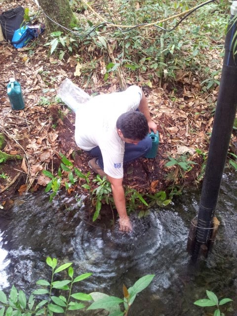
Sampling water samples direct from the stream (for control purposes) and storing them in an icebox for analysis within the following 24 hours.


At the laboratory in UFMT (Cuiabá). Filtering samples (vacuum pump) and doing TSS. The last picture is a scale we use to conduct a Phosphorus analysis when the sample has a very low P concentration.


When it is possible, I bring some instruments with problems back to the laboratory to repair and test them more appropriately.


Testing the equipment back in the field.


Collecting samples (each auto sampler has 24 bottles, and each bottle 1 liter of water) and labeling.


The usual scene: packing the car and transporting sand bags (each around 50 kg) to fix problems with the weirs.


At the weir: measuring and happy that is everything working fine :)


At the weather station, downloading the data.

Even the basics need to be done: soil texture analysis.


Collecting water from the overflow experiments at the Cropland catchment.


Doing a GPS survey in the gallery forests.


Machinery ready to harvest! And I was ready to collect water samples after it.


Two kinds of happiness: (a) work going well and (b) a good discovery, a small waterfall in the middle of a forest (with my snake protection) :)

Giving an interview for a local TV channel after a presentation at the Federal University of Mato Grosso.


Well, I hope you now have a good overview on my fieldwork activities in Brazil. Of course there is a lot more, most parts of the work are repeated daily (collecting data, installing/fixing instruments), but I tried to summarize it in way that you could see the most important aspects of it.

I would like to acknowledge to my supervisor and my research group (especially to Dr. Guzha), the group of soil sciences at UFMT (Federal Univ. of Mato Grosso) and other students, especially Jonas Macedo, Norma Bertao, Taciana Ziembowicz and Gilmar Torres, for all the excellent support in the lab and in the field.